An extensive Tutorial on Demographic Modeling with fastsimcoal2 Coalescent Simulations

fastsimcoal2 is a powerful Markov coalescent simulator, modeling complex evolutionary scenarios including shifting migration dynamics, effective population sizes, and population expansion or constrictions. These models can be specified by template files, permitting to introduce unknown parameter variables for estimation. Providing observed nucleotide data enables the iterative optimization of these estimated parameters by Brent algorithms aiming to increase the likelihood for the simulated data fitting the observed data. While this program is obtruse and requires precision in the file preparation, it is a precious addition to a biologist’s toolbelt. In this tutorial, I will provide a well-explained introduction to the most common use-cases of fastsimcoal2. For more complex scenarios or further information, check the original manual.

Preparation

To start anymodeling process with fastsimcoal2, it is best practice to define a Prefix, which will stay relevant throughout the analysis, and assign Deme numbers to each of your included population / species. Fastsimcoal always starts numbering from 0. Write these down as we will return to them shortly.
This could look something like:
PREFIX=Heller_Tutorial
#Demes (Populations)
species A = deme 0
species B = deme 1
hybrids = deme 2

Observed Site Frequency Spectra (SFS) are needed to improve parameter fit forthe model. There are two distinct types of SFS. Both require certain format changes to seamlessly work with fastsimcoal. I have presented these in this tutorial.

All SFS files provided to fastsimcoal must follow a strict naming convention. While easySFS automatically prepares these names in the fastsimcoal-folder, the ANGSD SFS files require a manual change. The names are dependent on the SFS state. For unfolded SFS (derived allele frequency), fastsimcoal2 expects:
“$PREFIX”_jointDAF1_0.obs, signifying the two-dimensional derived allele frequence between deme 1 and 0
Analogous, the folded SFS (minor allele frequency) is named by this pattern:
“$PREFIX”_jointMAF2_1.obs, describing the two-dimensional minor allele frequency between deme 2 and 1.

For multiSFS, which is a valid input type since fastsimcoal 2.6, the x-dimensional SFS should be named “$PREFIX”_DSFS.obs or “$PREFIX”_MSFS.obs for derived or minor allele frequency spectra accordingly.

While multidimensional SFS are great for simpler scenarios, these matrices can become increasingly complex to simulate with more than four demes involved. This might require switching to pairwise 2dSFS.

Template file

Once you have created all 2dSFS pairings or the multidimensional SFS and named them correctly, you can start to describe your evolutionary model in the "$PREFIX".tpl file. I propose to download a template file here and adjust accordingly, without implementing empty lines, tabs, symbols, or spaces. In the following subchapters, I will individually explain all relevant aspects of a complete template file for fastsimcoal2.

Careful: fastsimcoal2 is very sensitive to lettercases, spaces, empty lines, hidden symbols etc. Thus, a meticulous definition of your input file is required. Comments can be added via “//” and are ignored by the algorithm. Furthermore, variables can be defined freely but must avoid overlap with each other or functions of fastsimcoal2 itself. It is good practice to add dollar signs to the end of each variable, omitting overlap between variables like N_A and N_ANC.

Specify demes

First, we write the number of demes and their effective population sizes in the template file. If you did not previously estimate these parameters, you can give them a variable name. For scenario 1, this looks like this.

// Number of Demes throughout the model
2
// Effective haploid popuation sizes (diploid Ne * 2)
1000
N_2$

Then we describe the haploid sample sizes and generations since sampling. Haploid sample sizes relate to twice the number of your diploid samples, unless you use haplotype data. Usually, the sampling time of one population is set to 0 and used as an anchor unless there are observations between the last genomic sampling and the current state that ought to be included in the model (e.g., inferring the current status through the use of museum material). Generation times must be researched in the literature or inferred from life history parameters of the species.

// Haploid sample sizes and generations passed since sampling
20 0
20 0

Finally, we have to model growth rates of our populations. Note, that these are defined backwards in time. Hence, negative growth rates define a population expansion forward in time and vice-versa. Unless you choose restrictive priors, non-zero growth rates may introduce population size inflation or non-coalescence in models.

//Growth rates
0
0

Define Migration Matrices

After this, we can continue with defining our first migration matrices. This must equally be done with great care to only model migration between existing demes and not to itself. The migration matrix in fastsimcoal2 are Nij matrices with i and j being the number of demes. Like all events and dynamics in fastsimcoal2, migration matrices are specified backwards in time. So the recipient population receives migrants if you reverse the natural flow of time to how it is modeled. In chronological order, the recipient population is therefore the source and the donor population the sink of migrants. While this notation may confuse you at first, it is necessary to consider both perspectives. fastsimcoal2 defines the migration as the likelihood of genes from the source population ending up in the sink. By reversing time, it quantifies how many migrants of the recipient population’s Ne migrated per generation.

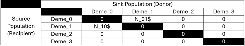
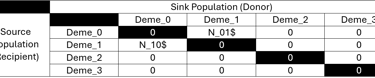
So in our scenario 1, we modelled an event, where 300 generations ago, a few individuals of C. bitaeniatus (deme 1) migrated towards the island Juan de Nova, home to C. caudatus (deme 0):

// Number of migration matrices
2
// Migration Matrix 0 :
0.000 0.000
N_10$ 0.000

As seen above, we defined two migration matrices. It is good practice to limit migration after (before in natural time progression) the divergence of species to prevent self-migration, hence we add:

// NoMig Matrix 1:
0.000 0.000
0.000 0.000

Include historical Events

Next, we must define our evolutionary events. As evolutionary events, we can define extinction events, migration pulses, divergence, or population size changes (e.g. sudden bottlenecks). Furthermore, these are useful to set changes in evolutionary dynamics as limiting migration after a certain period or changes in growth coefficients. Like the migration matrices, historical events are specified backwards in time. Consider that the time points of the events are defined by their defined time and not their order in the template.

This section is induced by adding the non-plural description "historical event" which is a part of the syntax and specifies how many following lines describe the historical events.The events are defined by the following space-delimited categories.

TIME_(GEN) SOURCE SINK MIGRATION NEW_DEME_SIZE NEW_GROWTH NEW_MIG_MATRIX

We now model the divergence scenario of deme 1 from deme 0 T_DIV$ generations ago. The source population is deme 0 with deme 1 as the sink. All genes of the source population (deme 0) merge with the sink (deme 1), the deme size does not change (1), neither does the growth rate (0). Finally, we switch to the NoMig Matrix (1) to avoid self-migration.

//Historical event: time (in gen), source, sink, proportion of migrants, new deme size, new growth rate, new migration matrix
1 historical event
T_DIV$ 0 1 1 1 0 1

Describe the Genome

Finally, we specify the number of unlinked blocks. To avoid errors, it is recommended to use 1 for the whole SFS and define it as following:
//Number of independent (unlinked) chromosomes, and "chromosome structure" flag: 0 for identical structure across chromosomes, and 1 for different structures on different chromosomes.
1 0
//Number of contiguous linkage blocks in chromosome 1:
1

SFS data is termed as FREQ, unless you have insights into recombination rates in your specimens, leave it at zero. It is preferable to have a simple than an overfitted model. The mutation rate can be derived for your focal group. E.g., for reptiles it is calculated to be 1.7e-8 and must not be 0 as otherwise divergence or similar processes leave no trace.
//per Block: data type, num loci, rec. rate and mut rate + optional parameters
FREQ 1 0 1.7e-8 OUTEXP

Estimation Files

Estimation files are required to specify model priors of the undefined variables from the template file. Priors are specified as a distribution information, a minimum, and a maximum value and must be stored in a file named as $PREFIX.est.
The tab-seperated columns are:

• Integer (1 = no, 0 = yes)

• Variable Name (as defined in $PREFIX.tpl)

• Distribution (uniform ("unif") or loguniform ("logunif"))

• Minimum Value

• Maximum Value

• "output" (if you provide this keyword, the estimated values are included in your output files)

• "bounded" (Meaning the model parameter cannot escape the prior spectrum)

• "reference" (to set one parameter as an anchor. I recommend to use the best researched information)
  

The file can look as following with the columns separated by single spaces.

[PARAMETERS]
//#isInt? #name #dist. #min #max
//all N are in number of haploid individuals
1 N_1$ logunif 100 10000 output
1 T_DIV$ logunif 1000 1000000 output

All that is left to do, is to run the model. Of course, you can vary parameters. However, I would be careful about being to non-restrictive as fastsimcoal2-models may be sensitive.

Practice examples

The most straightforward way to understand the mechanics and use of fastsimcoal2 is through modelling specific scenarios. Here, I simulated the SFS of several potential evolutionary scenarios that you might encounter during your research. They are a great introduction to the software and allow me to guide you step by step. Find all relevant files here. Alternatively, you may click on the title of each toy example to obtain the simulated datasets together with prepared template (.tpl), estimation (.est), and command (.sh) files.

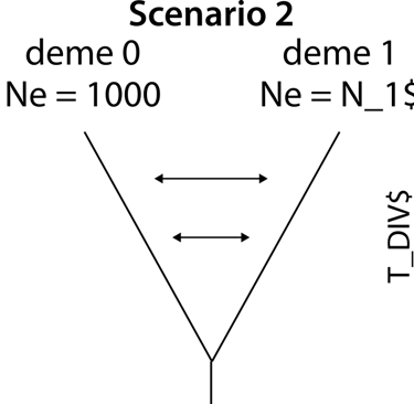
Scenario 1: Estimate Divergence and Effective Population Size (Ne)

A very common usecase of fastsimcoal2 is to estimate specific parameters such effective population sizes, migration, and divergence times. This scenario simulates a divergence of two demes (0 and 1) that have diverged X generations ago. While we know the effective population size of deme 0, we are unaware of the effective haploid population size of deme 1.
Thus, we use fastsimcoal2 to specify the following model, allowing the software to iteratively estimate our two unknown parameters, with this template (.tpl) file:

//Input parameters for the coalescence and recombination simulation program : simcoal2.exe
2
/Deme sizes (haploid number of genes)
1000
N_1$
//Sample Sizes
20 0
20 0
//Growth rates
0
0
//Number of migration matrices : If 0 : No migration between demes
1
//NoMig matrix 0 :
0.000 0.000
0.000 0.000
//Historical event: time (in gen), source, sink, proportion of migrants, new deme size, new growth rate, new migration matrix
1 historical event
T_DIV$ 0 1 1 1 0 keep
//Number of independent (unlinked) chromosomes, and "chromosome structure" flag: 0 for identical structure across chromosomes, and 1 for different structures on different chromosomes.
1 0
//Number of contiguous linkage blocks in chromosome 1:
1
//per Block: data type, num loci, rec. rate and mut rate + optional parameters
FREQ 1 0 1e-8 OUTEXP

In our simulated example, we know the effective haploid population size of 1000 for deme 0 (e.g., through linkage-based Ne inference), have 10 diploid samples from each deme (population) collected at the same time (20 0) , no population growth or migration (we need to specify a migration matrix nonetheless), 1 historical event T_DIV$-Generations ago where deme (0) diverged from deme (1) with 100% migrants (1) that did not influence the deme size (1) and did not change the growth rate (0) or the migration matrix (keep). The FREQ represents SFS data and 1e-8 represents an arbitrary mutation rate.
We have the simulated dataset Heller_Simulation_jointDAFpop1_0.obs for the observed derived allele frequency spectrum (DAF) between population 1 and 0.

We set the following broad prior estimation file (.est) as we have little knowledge about the exact parameters in this simulated sample. Both values are integers (1) and are suspected to have a loguniform distribution (logunif) between 100 and 1000000 and should be displayed in the output (output):

[PARAMETERS]
//#isInt? #name #dist. #min #max
//all N are in number of haploid individuals
1 N_1$ logunif 100 1000000 output
1 T_DIV$ logunif 100 1000000 output

Finally, we estimate the parameters with this command in the same directory. Here again, it is crucial to have the shared Prefix in all relevant files (.tpl, .est, _jointDAF1_0.obs).
fsc27093 -t Heller_Simulation.tpl -e Heller_Simulation.est -M -L 20 -n 100000 -d -I -x -y 3 -c 8 -q

This command specifies the path of fastsimcoal2 (fsc27093) with template (-t) and estimation (-e) files, 20 iterations (-L) of the Brent maximization algorithm, 100000 simulations per iteration (-n) on derived SFS (-d) with values resetting every three stagnant steps (-y) using 8 cores (-c) and a suppressed logging (-q).
After running fastsimcoal2, we see how quickly it converges to the values I used to simulate the model (N_1$ = 5000; T_DIV$ = 100000), despite the broadly set priors. The likelihood decrease indicates an increase in model fit.

fastsimcoal was invoked with the following command line arguments:
fsc27093 -t Heller_Tutorial.tpl -e Heller_Tutorial.est -M -L 20 -n 100000 -d -I -x -y 3 -c 8 -q

Random generator seed : 987703

No population growth detected in input file

Estimating model parameters using 12 batches and 8 threads

Estimation of parameters by conditional maximization via Brent algorithm (initial lhood = -1.46923e+07)
Iter 1 Curr best params: 3837 97743 lhood=-1.25942e+07
Iter 2 Curr best params: 5075 97743 lhood=-1.2587e+07
Iter 3 Curr best params: 5075 97743 lhood=-1.2587e+07

Scenario 2: Adding geneflow after divergence

We now repeat the same model as in scenario 1 but include and model geneflow after(!) the divergence of the two demes. In fastsimcoal2 terms, this requires a migration matrix in the beginning which shifts to a no-migration matrix after both demes merge. We specify now two migration matrices to avoid self-migration with migration from deme 1 to deme 0:

//Number of migration matrices : If 0 : No migration between demes
2
//Geneflow matrix 0 :
0.000 m_10$
0.000 0.000
//NoMig matrix 1 :
0.000 0.000
0.000 0.000

Und the historical events, we exchange "keep" with a shift to migration matrix 1:

1 historical event
T_DIV$ 0 1 1 1 0 1

And specify a reasonable prior range for migration in the Estimate-file (.est). Migration is always set between 0 (0%) and 1 (100%) and is thus a float value (0):

0 m_10$ unif 0 1e-4 output

And again, fastsimcoal2 converges within few steps to close estimates of the simulation parameters (N_1$ = 5000, T_DIV$ = 100000, and m_10$ = 1e-5) and then plateaus.

Estimation of parameters by conditional maximization via Brent algorithm (initial lhood = -1.23881e+07)

Iter 1 Curr best params: 1993 102787 1.05306e-05 lhood=-9.89865e+06
Iter 2 Curr best params: 4956 102787 1.05306e-05 lhood=-9.82823e+06
Iter 3 Curr best params: 4956 102787 1.03210e-05 lhood=-9.82820e+06
Iter 4 Curr best params: 4956 102787 1.03210e-05 lhood=-9.82819e+06

Scenario 3: Creating a new hybrid deme (population)

Finally, we are ready to create more complex models including generating new demes. In this scenario, we have our two diverging populations again which come into secondary contact and form a reproductively isolated hybrid population. We want to date this hybridization and estimate the initial interspecies proportions in this deme. We now specify the following three demes:

//Input parameters for the coalescence and recombination simulation program : simcoal2.exe
3
/Deme sizes (haploid number of genes)
1000
N_1$
100
//Sample Sizes
20 0
20 0
10 0

The hybridization event must be dated as following. The time (in gen) is unknown and will be estimated later. The source population (remember: specified backwards in time) is deme 2. First, hybridization event is the replacement of the hybrid deme with a specific proportion of migrants form 0 which does not change the deme size or growth rate, and then deme 1 provides the remaining hybrids (1) for the hybrid population so deme 2 ceases to exist (new deme size = 0).

//Historical event: time (in gen), source, sink, proportion of migrants, new deme size, new growth rate, new migration matrix
3 historical event
T_Hyb$ 2 0 m_Hyb$ 1 0 keep
T_Hyb$ 2 1 0 1 0 keep
T_DIV$ 0 1 1 1 0 keep

Again, fastsimcoal2 estimates the simulated values of (N_1$ = 5000, T_DIV$ = 100000, T_Hyb$ = 100, m_Hyb$ = 0.5) through quick convergence.

Estimation of parameters by conditional maximization via Brent algorithm (initial lhood = -5.11397e+06)
Iter 1 Curr best params: 6949 87166 97 0.5014373 lhood=-3763434.0006339
Iter 2 Curr best params: 4936 97668 97 0.5014373 lhood=-3758101.0267506
Iter 3 Curr best params: 4936 97668 97 0.5014373 lhood=-3758101.0267506
Iter 4 Curr best params: 4936 97668 98 0.5037411 lhood=-3758080.7005539
Iter 5 Curr best params: 4936 97668 98 0.5037411 lhood=-3758070.9161195
Iter 6 Curr best params: 4936 97668 98 0.4987037 lhood=-3758066.0339474

As shown by these three examples, the possibilities of fastsimcoal2 are vast. I am planning to include another tutorial on how to perform an automated parametric bootstrap in fastsimcoal2. All parameters in the evolutionary templates can be substituted by variables to be estimated through the coalescent simulations. If you have a request on how to model a specific scenario, feel free to contact me via the contact form.